Portfolio
Hey!
I’m Tam, an associate technical lead/senior software engineer with 5+ years of experience building low-latency, real-time systems in the AdTech industry
Featured Work
Here are some of the challenges I’m proud to have solved:
- Optimize: from 1800 to 800 cores
- Real-time Weather Augmentation
- Custom Routing for RTB
- Memory Profiling: Large Maps are Bad for Go GC
Tech Stack
- Languages:
- Golang: Deep understanding of goroutines, channels, mutexes, and GC internals
- Built services handling 40,000+ QPS, profiled and reduced GC pauses from large in-memory maps
- Large Maps are Bad for Go GC
- Custom Routing for RTB
- C++: Worked on RTBKit-based bidding engine, profiled Reactor event loops and tuned thread counts to match hardware config
- Python, Java
- Golang: Deep understanding of goroutines, channels, mutexes, and GC internals
- Databases & Messaging:
- Redis:
- Hit/miss caching with sorted sets and pipelining to reduce roundtrips: Real-time Weather Augmentation
- Lua scripts for atomic updates
- MongoDB:
- Ad-hoc queries to debug and find patterns for millions of requests, thousands of campaigns configuration
- Atomic task claiming for a distributed task queue: A Simple Task Scheduling System
- Kafka: Built producers in Golang with a goroutine pool, handled back pressure and errors
- Redis:
- Cloud & Infra:
- AWS: S3, SQS, EKS
- GCP: GCS, GKE
- BigTable: for real-time (sub-30ms) queries from golang client
- BigQuery: for ad-hoc analytics
- Kubernetes: statefulsets, deployments, auto-scaling, rollout management (up to 100-pod clusters)
- Observability & Networking:
- Grafana: built dashboards for debugging and monitoring production/qa/staging systems
- Prometheus: used counters, gauges, histograms from Golang client to measure request/error count and latency
- tcpdump: for low-level network debug
- Domains: Real-Time Bidding, Microservices, Geospatial (Uber H3, Google S2), Bitset-based filtering
Personal Projects
- Geoplot: A lightweight tool to visualize CSV files containing latitude and longitude data on a world map.
- Geodata: A tool to generate Uber H3 cell IDs, latitudes, and longitudes for all countries.
Contact
More Threads Can Harm Your Performance
TL;DR: By reducing the number of worker threads and unblocking our main event loop in a C++ Reactor-pattern system, we improved overall performance and downgraded our compute node from 36 cores to 16 cores. Across a deployment of 50 instances, this reduced our cluster from 1800 cores down to just 800 cores.
Introduction
In RTB (real time bidding) DSP (demand side platform) system, things move fast, usually the server must respond in 100ms. If it takes too long, it loses the auction.
I used to work on a RTB DSP system built with RTBKit, a fast C++ bidding engine. RTBKit is very powerful, but it has some tricky parts. Once, to handle more traffic, I simply added more worker threads. I thought using more CPU cores would mean more speed. But the opposite happened: our system became much slower.
This post explains why spinning up too many threads in a Reactor-pattern system can be bad, and how fixing it allowed us to improve performance significantly.
RTBKit Architecture
RTBKit uses a mix of thread pools and an event loop to process requests. The Event Loop sits in the center and routes messages between the different components. Here is a simple view of the system:
Worker ThreadsCPU-bound work
ThreadsIO-bound work
- Exchange workers: These are the main workers, they receive the HTTP bid request, parse the JSON, and match the bid request against a large number of campaigns. This is very CPU-intensive work.
- Event Loop: The exchange worker thread finishes and sends a message to a queue. The event loop picks it up and routes it to the augmenter threads.
- Augmenters: Add extra data to the request. IO-bound work.
- Bidders: Decide if they want to bid or not. IO-bound work.
- Send Response: The response routes back through the event loop to the exchange worker threads, which send it back to the ad exchange.
The Reactor Pattern and the Event Loop
In this system, components don’t call each other directly. They talk using queues. To tell another component that a message is ready, they use a single event loop. This is the Reactor Pattern. When a worker pushes a message to the queue, it wakes up the single event loop thread. The event loop reads the message and routes it to the right place.
This is a good design, but there is one weak spot: the single event loop thread. All messages must go through this one thread.
The Problem: adding too many threads
Our traffic was growing and requests started to timeout. Our server had 36 CPU cores per instance, so we thought: “We should add more exchange worker threads to utilize all these cores.” We increased our worker threads to match the available cores. We hoped the system would handle more requests.
Results: CPU usage got higher (which was expected, more cores joined the party), but request timeouts increased.
How could adding more workers make the system slower?
Debugging the Issue
We checked what the CPU was doing (with htop). Because you can set names for threads, we could see that the event loop thread was overloaded at maximum CPU. We added too many worker threads, so they were all parsing requests, matching campaigns, and sending messages to the event loop at the same time. The single event loop could not read and route messages fast enough
How We Fixed It
Fix 1: Remove work from the event loop
The Event Loop was running hot. In a Reactor pattern, we know the event loop should only route events, not actually do any work. So we hunted for any work inside the event loop. And we found that there were some “slightly slow” tasks, such as logging and data formatting, like this:
void EventLoop::dispatch(Message msg) {
    std::string logMsg = formatMetric(msg);
    logger.log(logMsg);
    targetQueue.push(msg);
}
These things only take a little time, but workers thread are pushing the event loop hard, so it adds up. We moved these non-critical work out of the event loop into the worker threads. After this change, performance slightly improved, which proved our point and built confidence a bit.
Fix 2: Reduce the worker threads
Then we scaled down the thread pool based on what the event loop could handle, more threads are not always better. We must match the thread count to our system’s architectural bottlenecks. We tested multiple configurations. By reducing the number of workers, the event loop had less pressure, and the system became noticeably faster. We discovered the sweet spot was using only 16 cores instead of 36 cores per instance. Across our deployment of 50 instances, this reduced our total footprint from 1800 cores back down to 800 cores, while maintaining better latency and higher throughput
Takeaways
- Thread tuning: More is not always better. Always test and find the best configuration for your system.
- Event loop design: Keep it fast. The event loop is only to route events. Never put even slightly slow code inside it.
Real-time Weather Augmentation
Our HTTP server handles global traffic and must respond in under 100ms end-to-end. A new feature request comes in: augment requests with local weather data before passing them to upstream processing. Weather context lets the upstream system make better decisions. A campaign for rain gear should bid higher when it is actually raining. The catch is that not all requests need this. Only requests from configurable target regions do, for example the US and EU.
The requirements are:
- Input: Each request has geographic coordinates (latitude and longitude)
- External API: Weather data comes from a third-party provider. It can take seconds to respond.
- Latency: Augmentation must finish in under 3ms
- Targeting: Only requests from targeted regions need weather data
We have two main challenges on the hot path:
- Checking whether a request needs weather data
- Fetching and attaching weather data within the latency budget
Challenge 1: Check if a request needs weather data
This happens for every HTTP request, so it must be very fast and predictable
The Naive Approach: Ray Casting
We can represent region boundaries as polygons and use a point-in-polygon algorithm like ray casting: cast a ray from the point to infinity and count how many edges it crosses. If the count is odd, the point is inside.
This is conceptually simple but breaks down in practice:
- Heavy CPU load: Country borders are complex. The US polygon alone can have thousands of edges. Checking each one on every incoming request is expensive at scale.
- Unpredictable latency: Computation time varies with polygon complexity and point location
The Optimized Approach: Uber H3
The problem with ray casting is that the work happens at request time. We fix this by doing the geometry work offline, before any request arrives.
We use Uber H3, a grid system that divides the globe into uniform hexagonal cells. Each cell has a unique 64-bit integer ID. Converting a latitude/longitude pair to a cell ID is fast and predictable
Offline Preprocessing:
We map our target region polygons (e.g. US, EU) onto the H3 grid at a chosen resolution. This gives us a set of cell IDs that cover the regions. We call this the Target Cell Set. At server startup, we load this set into memory as a Go map[uint64]bool.
Hot Path: When a request arrives, we convert its coordinates to an H3 cell ID. Then we check if that ID is in the Target Cell Set. The check is a single map lookup, O(1), no variance based on geographic complexity.
Building the Cell ID Set
We use geodata, a small open-source tool that generates H3 cell IDs for every country in the world. It reads country boundary polygons from Natural Earth GeoJSON data, fills each polygon with H3 cells at a given resolution, and writes the results to CSV files.
Performance Tuning: H3 Resolution
H3 resolution controls the size of each hexagonal cell. Higher resolution means smaller cells, better geographic precision, but more cells to store.
| Resolution | Avg Cell Area | Avg Edge Length | Approx. US cells |
|---|---|---|---|
| 3 | 12,393 km² | 68.98 km | ~2,000 |
| 4 | 1,770 km² | 26.07 km | ~14,000 |
| 5 | 253 km² | 9.85 km | ~97,000 |
| 6 | 36 km² | 3.73 km | ~680,000 |
We use resolution 5. At that resolution, the US is covered by roughly 97,000 cells. Each cell ID is a uint64 (8 bytes). A Go map[uint64]bool for the US at resolution 5 occupies roughly 10-15 MB including map overhead. That is cheap. We load the CSV at startup and keep it in memory for the lifetime of the process.
Weather targeting does not need street-level precision. An 10km edge length is accurate enough: weather is consistent within that radius, and the campaign targeting criteria are not that fine-grained. If requirements tighten, we can increase resolution without changing anything else in the system.
One further optimization is to use different resolutions for different regions. Dense urban areas might justify higher resolution for accuracy; sparse regions can afford lower resolution to save memory
Challenge 2: Augmenting Requests Without Blocking
Now we know the request is in the targeted region. Now we need to attach weather data in under 3ms. But the weather API takes seconds
Hit-Miss Cache with Background Refresher
The key insight is that weather data does not change per-request. Two requests from the same H3 cell within 15 minutes will see the same weather. We exploit this by caching weather data keyed by H3 cell ID, and refreshing it asynchronously in the background
The system has two parts: a fast hot path that reads from cache, and a background worker for the slow API calls.
The Hot Path Flow
When a request needs weather, we look up its H3 cell ID in Redis.
- Cache Hit: Attach the cached weather data. Done in a single Redis GET.
- Cache Miss: We cannot wait for the API. Instead, we record the missing cell ID using Redis
SADDinto a set calledcells_to_fetch, then forward the request upstream without weather data. The next request from the same cell will hit the cache after the background worker has filled it.
Using SADD is deliberate. If a popular location’s cache expires and thousands of requests arrive simultaneously, every one of them would write the same cell ID. Because cells_to_fetch is a Redis Set, duplicates are ignored automatically. The background worker will fetch that cell exactly once, not thousands of times.
cells_to_fetch
The Background Refresher
The Refresher is a dedicated service that runs on a 10-second tick. On each tick it:
- Pops up to 50 cell IDs from
cells_to_fetchusing RedisSPOP. - Converts each cell ID back to a representative latitude/longitude point (H3 supports this natively)
- Calls the weather API, using batch request to reduce network roundtrip
- Writes the results back to Redis with a TTL of 15min
After the refresher runs, subsequent requests from those cells will find their data in cache. The first request from a new location always misses. This is an acceptable trade-off
The batch size and tick interval are both configurable. Together they act as a soft rate limiter on external API calls.
Putting It All Together
map[uint64]bool (Target Cell Set)Key Takeaways
- Move heavy computation offline. Ray casting is correct but expensive and unpredictable. Precomputing the H3 cell set at build time reduces the hot path to a single integer lookup.
- Remove uncontrollable latency from the hot path. Anything that calls an external system at request time will eventually blow your budget. The background refresher owns the slow work; the request handler only reads from cache.
- Use data structures that match the access pattern.
SADDinto a Redis Set gives deduplication for free.map[uint64]boolgives O(1) lookup with no branching. Choose the right tool for each layer.
Custom Routing
Disclaimer: All numbers and examples in this article describe abstract ideas. They are not exact facts about any real system.
A RTB system handles 10,000 active campaigns, is horizontally scalable, we can add more compute nodes to handle more load. But scaling campaign capacity revealed a real problem: the more we scaled, the worse our match rate got.
The Problem: Campaigns Are Spread Thin
Matching a bid request to a campaign is CPU-heavy. For each incoming bid request, a node must check eligibility across every campaign: targeting rules, budget limits, frequency caps, and more. A single node cannot handle 10,000 campaigns at full traffic, so we distribute campaigns across nodes.
Each campaign is distributed across 3 of the 10 nodes (to increase visibility). That means each node holds about 3,000 campaigns:
Total campaigns: 10,000
Nodes: 10
Replicas per campaign: 3
Campaigns per node: 10,000 × 3 / 10 = 3,000
Incoming bid requests are routed to one node. That node only “sees” its 3,000 campaigns. If the right campaign for this request lives on one of the other 7 nodes, we waste that request
As we added more nodes to scale capacity, campaigns were spread even thinner across them. The match rate got worse. This is a fundamental issue with round-robin routing. The load balancer distributes requests evenly across nodes with no awareness of which campaigns each node holds, so no node has visibility of all campaigns
The Solution: A Custom Reverse Proxy
We built a reverse proxy that sits in front of the compute nodes. Instead of round-robin routing, it routes each bid request to the node most likely to have a matching campaign. The proxy does not run the full filtering logic, that is too CPU-heavy. Instead, it applies a small number of fast, lightweight filter, the goal is to remove clearly wrong nodes and increase the probability that a bid request lands on a node with a matching campaign
We built this in Go using the standard net/http/httputil.ReverseProxy package with custom routing logic, pre-computed routing data is stored in Redis. We store this data in Redis instead of Go’s memory, because keeping millions of entries in a map[string]string inside a Go process puts heavy pressure on the garbage collector. Go’s GC must scan every pointer in the map on every cycle, which causes periodic CPU spikes. Moving the data to Redis removes it from Go’s heap entirely. We covered this issue in detail in Large Maps Are Bad for Go GC, which we discovered while building this proxy.
How the Routing Works
When a bid request arrives at the proxy:
- Read key attributes from the request (e.g. userID)
- Look up those attributes in Redis to retrieve the pre-computed list of candidate nodes
- Randomly pick one node from that list and forward the request
We only apply fast filter checks, the ones with high selectivity and low compute cost. The full filtering still happens on the compute node
Upstream Health Checks
At first, we only checked whether upstream nodes were alive. If a node stopped responding to health checks, we removed it from the routing pool. Then we found that when a node crashes and restarts, it comes back online healthy but has no active campaigns yet because it has not finished loading its campaign data. This becomes a problem when the proxy uses least request routing. An empty node responds to requests very fast because it has nothing to check, so it always appears to have the fewest in-flight requests. The proxy keeps sending it more traffic, which all result in no bid
We then exposed an API endpoint that returns its current active campaign count, the proxy checks this count. If it is zero (or below a minimum threshold), the node is skipped from the routing pool until it is ready
Results and Trade-offs
After deploying the custom routing proxy, our match rate increased by around 30%. The trade-off is added latency. The proxy needs to query Redis and run routing logic before forwarding. This adds around 5ms to each request, which is acceptable in our systems
Key Takeaways
- Do lightweight filtering at the proxy layer. Running full filtering at the proxy is too expensive. A few fast checks are enough to make better routing decisions
- Healthy does not mean ready. A node that just restarted can appear healthy but have no data. Check application-level readiness, not just network-level liveness
Large Maps Are Bad for Go GC
How Go GC Works
Go uses a concurrent mark-and-sweep garbage collector. During every GC cycle, the runtime has to figure out which objects in memory are still being used (live) and which can be safely thrown away. It does this in two main phases:
- Mark phase: The GC starts from “roots” (like global variables and stack variables) and traces every pointer it can find. If it finds a pointer to an object, it marks that object as “alive”. It keeps following pointers from object to object until everything reachable is marked.
- Sweep phase: The GC goes through memory and reclaims any space occupied by objects that were not marked as alive.
The critical thing to understand here is that the cost of the mark phase scales with the number of pointers it has to scan, not the raw number of bytes in memory.
If you have a 1 Gigabyte array of pure bytes ([]byte), the GC looks at it, sees there are zero pointers inside, and moves on immediately. It takes almost zero time.
But if you allocate 1 Gigabyte of small objects linked together by millions of pointers, the GC has to chase down every single one of those pointers. That takes a lot of CPU cycles and pauses your application.
This is a well-known issue in the Go community: runtime: Large maps cause significant GC pauses
Large Map in Go
Let’s look at map[string]string. When you create a map with millions of entries, you might think you are just storing keys and values. But under the hood, a Go map is a complex hash table.
A map[string]string contains:
- A pointer to the internal
hmapstruct (the header). - Pointers to an array of buckets. Each bucket holds up to 8 key-value pairs.
- Overflow buckets, which are linked lists of extra buckets if there are collisions.
- For each entry in the map, there is a key and a value.
A string in Go is not just a blob of text. Under the hood, a string is a struct containing two things: a pointer to the actual underlying byte array, and an integer for the length.
So, if you have a map[string]string with 10 million entries, you do not just have 10 million items. You have:
- Millions of internal bucket pointers.
- 10 million pointers for the keys (the string headers).
- 10 million pointers for the values.
That is over 20 million individual pointers! During every single GC cycle, the Go standard garbage collector must scan all of them.
ptr + len
ptr + len
Even if you never modify the map, the GC does not know that. It has to scan the whole thing every time to make sure memory is still reachable
The case: The high-traffic HTTP reverse proxy
I once worked on an HTTP reverse proxy service written in Go. Its job was to apply custom routing logic, mapping incoming requests to correct upstream services. I describe the routing system in detail in Custom Routing. This GC issue is one of the things I ran into while building it:
- We ran 10 nodes, each with 4 CPU cores.
- Each processes ~4,000 queries per second (QPS), payload is ~3KB JSON
To make routing fast, we decided to load all the routing rules into a map[string]string when the process started. It worked beautifully at first. But over time as the routing rule set grew, and things got weird. We noticed periodic CPU spikes across the nodes. At first, the Prometheus monitoring charts looked okay because metrics were averaged over a 5-minute interval, which smoothed out the spikes
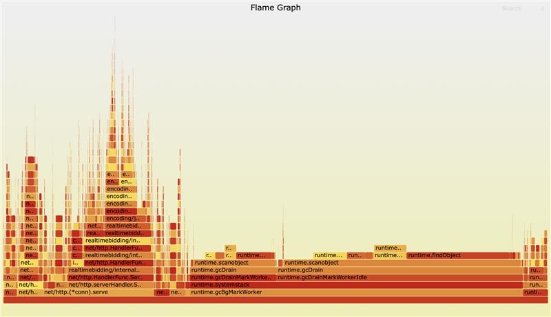
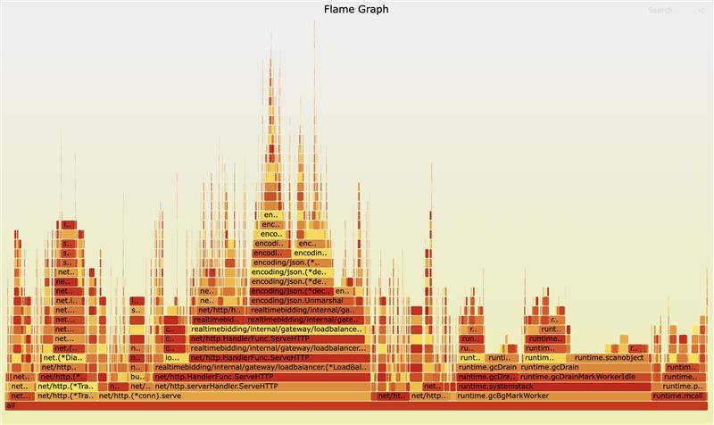
Then I used pprof to see where the CPU time was going. I expected to see JSON parsing taking up the time. Instead, I saw runtime.gcDrainMarkWorker and runtime.gcDrainMarkWorkerIdle dominating the CPU profile. The GC was working overtime just to check a large map what would never run out of scope
Here is the workflow of the old system:
map[string]string, millions of pointers, lives forever in GC scope
Reproducing the Issue
To prove this was the root cause, I wrote a simple script to benchmark the GC pause time with different map sizes.
package main

import (
	"fmt"
	"runtime"
	"time"
)

func run(n int) {
	// Pre-allocate the map to avoid resizing cost during setup
	routes := make(map[string]string, n)

	// Populate the map with n items
	for i := range n {
		routes[fmt.Sprintf("key-%d", i)] = fmt.Sprintf("value-%d", i)
	}

	const runs = 10
	var totalPause time.Duration

	// Trigger GC manually and measure how long it takes
	for range runs {
		start := time.Now()
		runtime.GC()
		pause := time.Since(start)
		totalPause += pause
	}

	avgMs := float64(totalPause.Milliseconds()) / float64(runs)
	fmt.Printf("n=%d | avg GC pause=%.3fms\n", n, avgMs)

	// Prevent the map from being garbage collected by compiler optimization
	_ = routes["key-0"]
}

func main() {
	run(1_000_000)
	run(10_000_000)
	run(20_000_000)
}
Running this script gave very clear results:
% go run ./...
n=1000000 | avg GC pause=10.200ms
n=10000000 | avg GC pause=103.300ms
n=20000000 | avg GC pause=342.600ms
As you can see, the GC pause time grows linearly with the number of items in the map. A 342ms pause in a system that requires sub-100ms latency is an absolute disaster.
And here’s the real flame chart:
Finding a Solution
Approach 1: Off-Heap Caching Libraries
I considered using libraries like BigCache or FreeCache. These libraries avoid GC overhead by allocating large byte arrays (which have no pointers) and managing the memory layout themselves
Approach 2: External Store (Redis)
Instead of keeping the data in memory, why not move it out of the Go process entirely? Redis is built exactly for this use case. By moving the routing rules to Redis, we would completely remove the data from Go’s memory space, freeing the GC.
We go with Redis
Both solutions sound good, and we decided to go with Redis. Because it also reduce whole system memory. The new workflow looks like this:
data lives outside Go heap, invisible to GC, adds ~2ms latency
The results:
- GC pauses dropped significantly
- Overall RAM usage decreased: Instead of keeping duplicated data across 10 Go nodes, we kept a copy in Redis. This saved us a lot of infra cost
- Latency trade-off: Redis adds ~1-2 milliseconds, which is acceptable
Takeaways:
- Profile early and often
- Avoid large maps with pointers
- Consider external stores
We must discard unread body in Golang
Out of the box, Go’s http.Client is built for high performance. It uses a component called http.Transport to manage a pool of underlying TCP connections.
When a service makes a request to an external API, the Transport checks the pool to see if there is an idle connection waiting to be reused. If there is, it sends the request over that existing connection. This is HTTP Keep-Alive in action. Reusing connections saves the heavy cost of DNS resolution, TCP handshakes, and TLS setup.
When a service finishes reading a response and calls resp.Body.Close(), the Transport takes that connection and puts it back into the pool.
But there is a catch. The connection can only be reused if the server has finished sending the response and the client has finished reading it. If there is leftover data on the wire, the connection is considered “dirty.”
Sometimes, we only care about the HTTP status code. For example, maybe we are pinging a health check endpoint or sending a fire-and-forget webhook. We write something like this:
resp, err := client.Post("https://api.example.com/webhook", "application/json", body)
if err != nil {
    return err
}
defer resp.Body.Close()

// The response body is not needed here; only success status matters.
if resp.StatusCode != http.StatusOK {
    return fmt.Errorf("unexpected status: %d", resp.StatusCode)
}

return nil
Because we did not read the response body to the end, the Go standard library does not know what is still sitting on the incoming network buffer. To prevent corrupted reads for the next request that might try to use this connection, the http.Transport permanently closes the underlying TCP connection and throws it away. As a result, the connection pool becomes useless. For every single request, it establishes a brand new connection.
Proving it with Benchmarks
This can be proven with a simple benchmark. A local HTTP server is set up to return a payload. Then, the httptrace package is used to hook into the GotConn lifecycle event. This tells exactly if a connection was freshly created or reused from the pool.
(Note: Source code for this benchmark is available here)
func doBench(b *testing.B, discard bool) {
	server := setupServer() // Returns an HTTP server sending 32KB of data
	defer server.Close()

	client := &http.Client{}
	var created, reused int

	for b.Loop() {
		trace := &httptrace.ClientTrace{
			GotConn: func(connInfo httptrace.GotConnInfo) {
				if connInfo.Reused {
					reused++
				} else {
					created++
				}
			},
		}

		req, _ := http.NewRequest(http.MethodGet, server.URL, nil)
		req = req.WithContext(httptrace.WithClientTrace(req.Context(), trace))

		resp, err := client.Do(req)
		if err != nil {
			b.Fatal(err)
		}

		// The critical difference
		if discard {
			io.Copy(io.Discard, resp.Body)
		}
		resp.Body.Close()
	}
	b.Logf("Connections Created: %d, Connections Reused: %d", created, reused)
}
Result:
BenchmarkHTTPDiscard
    main_test.go:72: Connections Created: 1, Connections Reused: 25208
BenchmarkHTTPDiscard-8             25209             46355 ns/op           38582 B/op         69 allocs/op
BenchmarkHTTPNoDiscard
    main_test.go:72: Connections Created: 11319, Connections Reused: 0
BenchmarkHTTPNoDiscard-8           11319            106628 ns/op           51070 B/op        131 allocs/op
Summary
When working with net/http in Go, we should never assume defer resp.Body.Close() is a complete solution:
- We must read the body to EOF
- Use
io.Copy(io.Discard, resp.Body)to safely flush unwanted bytes
Building a Simple Distributed Task Scheduling System
In this post, I will describe a simple, horizontally scalable distributed task scheduling system using just Go and MongoDB. For what purpose, I can’t say. But it works.
System requirements:
- Unpredictable Workloads: All tasks must be executed. A task can take anywhere from 2 seconds to 10 minutes.
- Horizontal Scaling: The system scales simply by adding more worker nodes.
- Simplicity: Adding new nodes or tasks must be straightforward.
The system has three components:
Task Handler:
This acts as the controller and performs the following tasks:
- Fetches new tasks from external sources.
- Inserts them into the MongoDB with a
pendingstatus. - Scans MongoDB for tasks with a
donestatus and sends the results to external services. - Scans MongoDB for tasks with a
workingstatus to check if they are overdue (say, 15 minutes). If they are, it resets their status topending.
Worker:
This component does the heavy lifting and performs the following tasks:
- Polls MongoDB for tasks with a
pendingstatus. - Claims a task by atomically changing its status to
workingusing MongoDB’sfindOneAndUpdate. - Finishes the work and saves the result to the document, updating its status to
done.
MongoDB:
It’s MongoDB 😏. It handles atomic operations and storage.
Matrix-Based Filtering
The Matching Problem
In a Real-Time Bidding (RTB) system, a Demand-Side Platform (DSP) handles thousands of bid requests every second. For each request, we must quickly find which active campaigns want to bid on it.
Each bid request has multiple attributes, like country (“us”, “jp”, “sg”), language (“en”, “fr”, “vn”), device type, and website. At the same time, each campaign has strict targeting rules. One campaign might only target iOS users from the “us” who speak “en”. Another might accept users from anywhere except the “eu”.
We only have ~100ms to find all matching campaigns. A simple approach is to loop through every campaign and check its rules one by one. But this is too slow. Checking 50 rules for thousand of campaigns for every request takes too much time.
A better approach is to use a matrix-based filtering approach. Instead of checking a request against each campaign, we use an inverted index. This means we map request attributes directly to the campaigns looking for them.
The Matrix-Based System
The matching logic uses bitsets. A bitset is an array of bits (0s and 1s). Every campaign gets a fixed ID. In a bitset, the bit at index i always stands for campaign i. And we do not store rules inside campaign objects. Instead, we use separate filters for each attribute, like a Language Filter or a Location Filter. Each filter manages its own include and exclude rules using maps. The map key is the attribute (like “en” or “us”), and the value is a bitset. We evaluate these rules based on simple logic:
- No include, no exclude: accept all values.
- No include, has exclude: accept all values except those in exclude list.
- Has include, no exclude: accept only values in include list.
- Has include, has exclude: accept only values in include list, that are not in exclude list
To do this fast, each filter keeps three things:
include_map: Maps a value to a bitset of campaigns that want it.exclude_map: Maps a value to a bitset of campaigns that block it.empty_include_bitset: A single bitset of campaigns that have no include rules (so they accept anything by default).
Evaluating a Filter
When a bid request comes in with language=“en”, the Language Filter does a fast look-up.
First, it gets include_map["en"] and combines it with empty_include_bitset using a bitwise OR. This gives us a bitset of all campaigns that accept “en”.
Second, it gets exclude_map["en"].
Finally, it removes the excluded campaigns using a bitwise AND NOT. We can write this as one simple formula to find the valid campaigns:
(include_map["en"] OR empty_include_bitset) AND NOT exclude_map["en"]
This simple math lets us check the rules for all campaigns at the exact same time.
Combining the Rules
When a bid request starts, we create a main bitset called active_campaigns. We set all bits to 1 because all campaigns start as valid choices. Then, we check each filter. After a filter gives us its result bitset, we use a bitwise AND on active_campaigns to update the state.
Performance Benefits
First, we skip the slow loop over all campaigns. The time it takes now depends only on how many attributes the bid request has, not how many campaigns we run. This keeps the system fast even when we add many more campaigns.
Second, looking up items in a map is very fast. Using bitwise math updates every campaign instantly in O(1) time.
Finally, bitsets use very little memory. We can track many campaigns with just a few bytes. Because it is so small, it fits perfectly inside the fast CPU cache.
Reference:
- https://github.com/rtbkit/rtbkit/wiki/Filter
Mapping Country Boundaries to H3 Hexagonal Grids
Many geospatial systems need to check whether a user’s location falls within a target region. One common approach is to store country boundaries as polygons, then run a point-in-polygon query at runtime. This works, but polygon containment checks are expensive, especially when you run them millions of times per second across thousands of campaigns
A better approach: precompute the answer. Convert each country boundary into a set of discrete cell IDs. At query time, you only need to check if a cell ID is in a set, which is a fast hash lookup
geodata is a small Go tool that does this precomputation. It takes country boundary polygons from Natural Earth and fills them with Uber H3 hexagonal cells, writing the results to CSV files
What Is H3?
H3 is Uber’s open-source hexagonal grid system. The globe is divided into hexagonal cells at multiple resolutions. Each cell has a unique 64-bit integer ID. At resolution 4, each cell covers about 1,770 km2. Higher resolutions give finer granularity but more cells per country
Hexagons are a good fit for this use case because they tile the plane uniformly. Every cell has six equidistant neighbors, so there is no directional bias when querying nearby cells
How It Works
The tool does three things: fetch country boundary polygons, fill each polygon with H3 cells, and write the results to CSV
Fetching Country Polygons
The GeoJSON source is the Natural Earth 1:110m admin-0 dataset, fetched directly from GitHub at startup. Natural Earth is a public domain dataset widely used for cartographic work. The tool falls back to a local copy in the repository if the download fails
Each GeoJSON feature maps to one country. The code reads the ISO_A3 property as the country identifier. Some countries in the dataset have -99 as their ISO_A3 value (a Natural Earth convention for disputed or unmapped territories), so the code falls back to the ISO_A3_EH property and validates it against a countries library before accepting it
Filling Polygons with H3 Cells
The core operation is h3.PolygonToCells(polygon, resolution). This returns all H3 cells whose centers fall within the given polygon at the requested resolution
Many countries have non-contiguous territories: islands, overseas regions, exclaves. In GeoJSON these appear as MultiPolygon geometries. The code handles this by iterating over each sub-polygon separately and collecting cells from all of them into a single map. The map serves as a deduplication set, since adjacent polygons might produce the same border cells
Country A (MultiPolygon)
  ├── Polygon 1 (mainland)  → cells {a, b, c, d}
  ├── Polygon 2 (island 1)  → cells {e, f}
  └── Polygon 3 (island 2)  → cells {d, g}   ← d is a duplicate
                                               → final: {a, b, c, d, e, f, g}
Output Format
Each country gets a CSV file named h3_res_{resolution}_{iso_a3}.csv with three columns:
id,lat,lng
599690792927657983,52.765347,5.199402
599693744560906239,52.388095,4.899597
...
The id column is the H3 cell ID as a uint64. The lat/lng columns are the cell’s center coordinates, computed by cell.LatLng(). These can be loaded directly into a geospatial database or visualized with a tool like geoplot
Using the Output
The intended use is geo-targeting: load each country’s cell set into a key-value store or in-memory set, then at query time convert the user’s coordinates to an H3 cell ID at the same resolution and check membership
user location (lat, lng)
  → h3.LatLngToCell(lat, lng, resolution)  → cell ID
  → set.Contains(cellID)                   → true/false
This replaces an expensive point-in-polygon computation with a single hash lookup. The trade-off is coverage at borders: cells are discrete, so a cell on the boundary of a country may or may not be included depending on where its center falls. At resolution 4, each cell is about 1,770 km2, so the maximum border error is on the order of one cell width (~42 km). Higher resolutions reduce this error at the cost of more cells per country
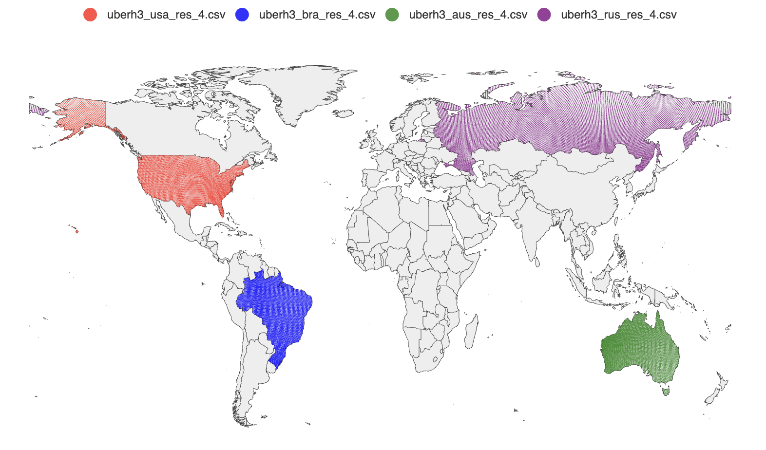
Visualizing Geospatial CSV Data with geoplot
When working on geodata, we needed a way to verify the output: are the H3 cells actually covering the right countries? Eyeballing raw CSV files with thousands of lat/lng rows is not practical. We needed to plot them on a map
geoplot is a small Go HTTP server that reads CSV files and renders their coordinates as scatter points on an interactive world map. You pass it file names via query parameters, it serves back a rendered map in the browser
How It Works
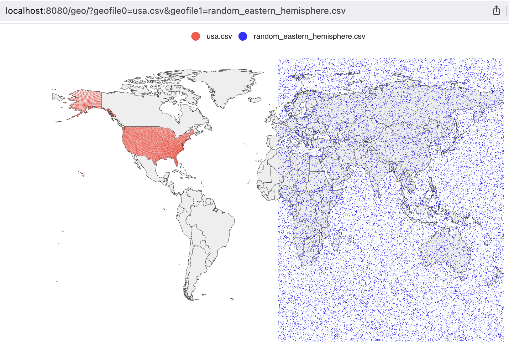
The server exposes a single endpoint: /geo/. You specify up to 100 CSV files via query parameters geofile0, geofile1, and so on. Each file is loaded, parsed, and rendered as a separate series on the map with a distinct color
http://localhost:8080/geo/?geofile0=usa.csv&geofile1=latlon.csv
Column Auto-Detection
The CSV parser does not require a fixed column order. It scans the first data row and finds the first field that parses as a valid latitude (a float between -90 and 90). That column index is stored and reused for every subsequent row. The column immediately to its right is treated as longitude
This means it works with CSV files that have leading ID columns, like the output from geodata:
id,lat,lng
599690792927657983,52.765347,5.199402
The id field is not a valid latitude, so the parser skips it and correctly identifies lat as column 1
Rendering
The chart uses go-echarts, which wraps Apache ECharts. Each file becomes a named scatter series. Points are sorted by latitude before rendering, which does not change the visual output but makes the series consistent across reloads. The map is interactive: you can zoom and pan in the browser
Colors cycle through a fixed list (red, blue, black), assigned by file index. The file name is used as the series label, so it appears in the legend
Car Simulator
Car simulator is a simple HTML program for practicing horizontal and vertical parking